Formal Verification for LLM Reasoning: Solvers and Theorem Provers

Introduction

In the previous post, the judge of a chain of thought was a reward model: another neural network that reads a solution and scores it. A reward model can be wrong, and a policy trained against it can learn to fool it. For some kinds of reasoning there is a judge that cannot be fooled: a program that checks the reasoning by the rules of logic. If the reasoning is written in a formal language, a solver can compute what follows from it, and a proof assistant can check every step of a proof. The answer is not a probability but a yes or a no, and a yes is guaranteed to be right.

The catch is that the model must now write in that formal language, which is much harder than writing natural language. LLMs have seen little of it during pre-training, the syntax is strict, and one wrong symbol makes the whole thing fail. This post goes through twelve recent papers that put a formal checker in the loop with an LLM. The first two use a checker to guide ordinary reasoning: an answer set programming solver that checks partial programs for logic puzzles, and a logic solver that checks steps inside a chain of thought. The other ten are about theorem proving, where the LLM writes proofs in Lean, Isabelle or Coq and the proof assistant checks them. We first set up the basic vocabulary of proof assistants, then look at the solver papers, and then at the provers: how they find the right facts, how they learn from step-level feedback, how they repair failed proofs, how one very large prover is trained, and how provers handle problems where the answer or even the statement is not given.

How a Proof Assistant Checks a Proof

The theorem-proving papers all share the same basic setting, so we set it up once here. A proof assistant, also called an interactive theorem prover, is a program that checks mathematical proofs written in its own language. The papers here use three of them: Lean 4, with its large library of formalized mathematics called Mathlib; Isabelle/HOL; and Coq, recently renamed Rocq. A short Lean proof looks like this:

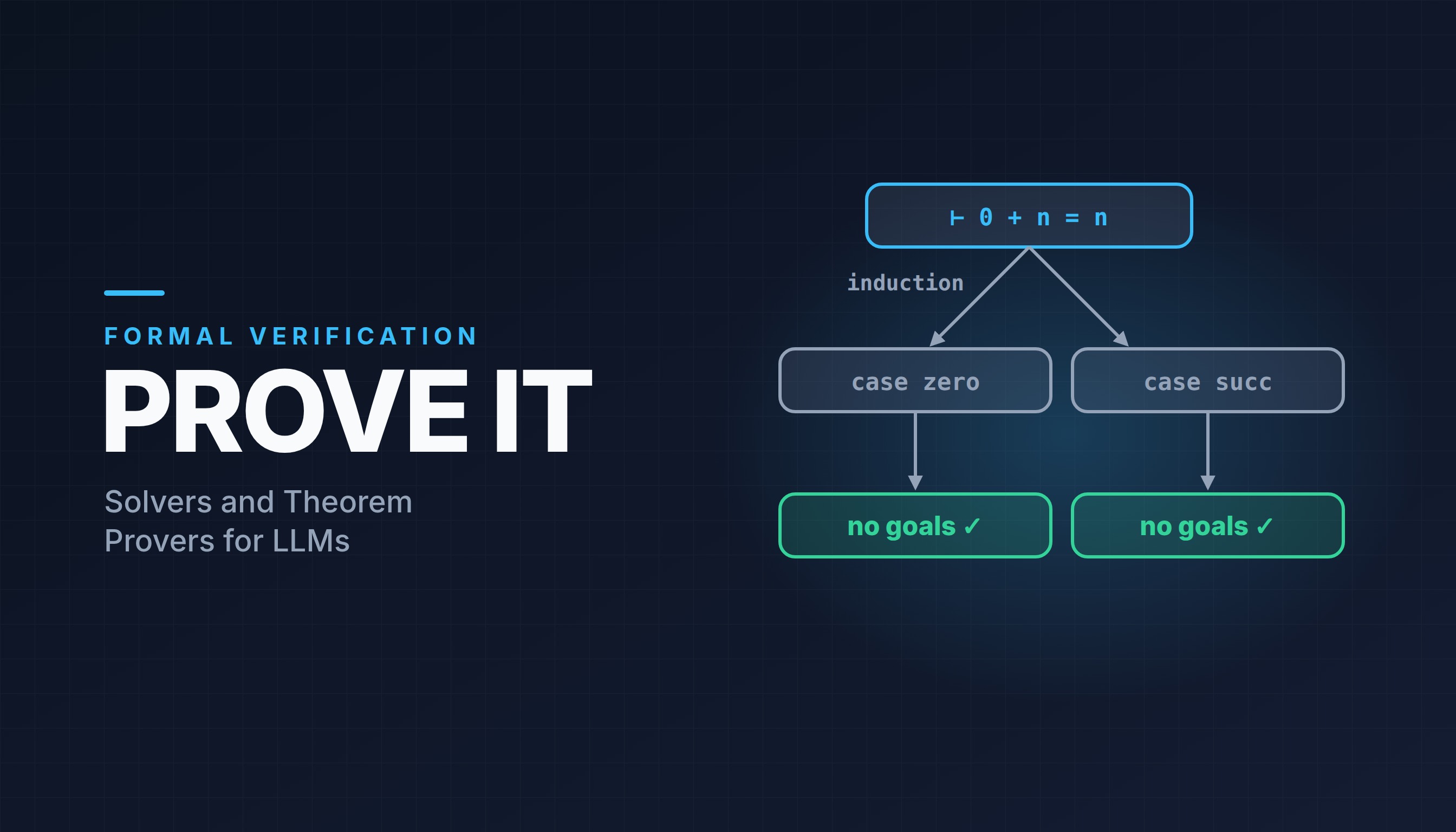
theorem zero_add_example (n : Nat) : 0 + n = n := by
  induction n with
  | zero => rfl
  | succ n ih => simp [ih]

The first line is the theorem statement. After by comes the proof, written as a list of tactics. A tactic is a command that changes what is left to prove. At every moment, the proof assistant keeps a proof state: the list of goals still to be proved, each with the facts that can be used for it (Figure 1). The tactic induction n turns one goal into two, a base case and an inductive case with the induction hypothesis ih. The tactic rfl closes the first goal, and simp [ih] closes the second. When no goals are left, the theorem is proved.

If a tactic does not apply to the current goal, the proof assistant reports an error. This is what makes it a perfect checker: every step is either accepted or rejected, and the final proof is checked by a small trusted part of the system called the kernel. Two more words appear often. A premise is an existing lemma or definition that a tactic uses, like ih above or a lemma from Mathlib. And sorry is a placeholder that says “assume this part is proved”. A proof that contains sorry is accepted for its structure but is not complete. Lean and Isabelle use the same word, and many methods below use sorry to mark the parts that are still missing.

There are two ways to prove a theorem with an LLM (Figure 2). In tactic-by-tactic proving, the model reads the current proof state and proposes the next tactic, the proof assistant runs it, and a search builds a tree of proof states until one with no goals is found. In whole-proof generation, the model writes the entire proof at once, and the proof assistant either accepts it or reports where it fails.

The most common search for tactic-by-tactic proving is best-first search. The model proposes several tactics for a proof state, usually with beam search, and each tactic that the proof assistant accepts creates a new state. The search keeps a queue of states and always expands the one whose path is most likely under the model. A state $s$ reached by the tactics $a_1,\dots ,a_k$ from the states $s_0,\dots ,s_{k-1}$ has the score

where $\pi (a\mid s)$ is the model’s probability of writing tactic $a$ in state $s$. The search stops when it finds a state with no goals, or when it runs out of time.

Solvers in the Loop

A solver does not need a proof. Given a set of rules and constraints in its own language, it computes every answer that satisfies them, or proves that none exists. This makes it useful for reasoning that is not written as a theorem. The LLM translates a problem into rules, and the solver does the reasoning. The two papers in this section use a solver to check not only the final program but also the parts the model writes along the way, and they turn the solver’s answers into training data and rewards.

An ASP Solver in the Loop

Schrader et al. [1] teach LLMs to write answer set programming (ASP). ASP is a language for combinatorial search problems such as scheduling and assignment. An ASP program has rules and constraints, and an ASP solver, here clingo, computes its answer sets: the sets of facts that satisfy all of them. Take a puzzle in which three dogs are walked by three people at three different times. The program first declares the entities and a choice rule that generates every possible assignment:

dog(beagle;golden;bernese). person(tom;eva;anna). time(8;9;10).
1 { walk(D, P, T) : dog(D), person(P) } 1 :- time(T).

The second line says that at each time $T$, exactly one dog $D$ is walked by one person $P$. Each hint of the puzzle then becomes a constraint. “Anna walks her dog later than Eva” becomes

:- walk(_, anna, T1), walk(_, eva, T2), not T1 > T2.

which rules out every assignment where Anna’s time is not later than Eva’s. ASP has a useful property for checking: adding a constraint can only remove answer sets, never add new ones. So a partial program can be checked on its own. If it still has the true solution among its answer sets, it is on the right track. If it has lost the true solution, a mistake has already been made.

A puzzle is written as $I=(D,E,H,S)$: a description $D$, the entities $E$, the hints $H=(h_1,\dots ,h_n)$ and the solution $S$. The LLM writes the program one piece at a time. It first writes the encoding ${\Gamma }_{C,E}$ of the entities and the choice rule, then one encoding ${\Gamma }_k$ for each hint $h_k$. This gives a trajectory of inputs and outputs:

where $P_{D,E}$ is the prompt with the description and the entities. At each step $k$, five continuations ${\Gamma }_k$ are sampled, and the solver is run on the partial program ${\Gamma }_{C,E}\cup {\Gamma }_1\cup \cdots \cup {\Gamma }_k$ (Figure 3). A continuation is chosen if the true solution is still among the answer sets:

where $\text{AS}(\cdot )$ is the set of answer sets computed by the solver. It is rejected if the solver reports an error, if the program has no answer sets at all (it is unsatisfiable), or if all of its answer sets are wrong. Only the problem description and its solution are needed, no hand-written ASP.

The chosen continuations become training data. With ${\mathcal{D}}_{\text{chosen}}$ the set of pairs of an input trajectory ${\mathcal{T}}_k$ (everything up to hint $h_k$) and a chosen continuation ${\Gamma }_k$, the model is trained with supervised fine-tuning (SFT):

The chosen and rejected pairs could also be used for DPO, but the authors found that plain SFT worked slightly better.

At test time the true solution is not known, so the solver’s output is turned into a reward instead. For an encoding $\Gamma$ with $M$ answer sets, the reward is

where $1_E$ is $1$ if the solver reports errors or warnings, $1_U$ is $1$ if the program is unsatisfiable, and $1_{NE}$ is $1$ if the number of answer sets is above a fixed limit, which protects against broken programs that explode. Each hint should narrow down the answers, so the term $1/M$ prefers stricter programs: a program with one answer set gets the largest reward. The search is greedy. For each hint, it samples $N$ continuations, keeps the one with the highest reward, and moves on. If all $N$ get a negative reward, it first samples $2N$ more, and if those fail too, it backtracks to an earlier hint that had other good options (Algorithm 1).

For the choice rule, the reward of Eq. (5) is replaced by a strict check: an $m\times n$ grid puzzle with no constraints has exactly $(n!{)}^{m-1}$ answer sets, so the encoding must produce that many. In the dog puzzle, $m=n=3$ and the choice rule must give $(3!{)}^2=36$ answer sets. After fine-tuning on data generated by Llama-3.3 70B, 8B models that could barely write ASP before improved by about 20 to 25 points on the puzzles.

Formal Logic Checks Inside a Chain of Thought

The ASP paper replaces natural-language reasoning with a program. Cao et al. [2] keep the natural language and add formal checks to it. Their formal logic verification (FLV) framework trains a model to write a natural-language step, then a short formal check of that step in a language such as Python with the Z3 solver, then to read the result of running it, and then to continue. Figure 4 shows the example from the paper. A chain of thought concludes from “Alice > Bob, Charlie < Alice, Diana > Charlie” that Diana scores higher than Bob. The model writes a Z3 check, the solver finds a counterexample in which Bob scores higher, and the next step corrects the conclusion: the facts do not decide the order.

A training example interleaves $N$ modules. Each module is a natural-language step $s_k$, a formal check $f_k^{\prime }$ inside <code> tags, and the actual output $v_k^{\text{act}}$ of running it inside <interpreter> tags:

where $\oplus$ means joining text one after another. Such data does not exist, so it is built. A teacher model writes four chains of thought per problem, and only chains with a correct final answer are kept. An LLM splits each chain into modules and writes a formal check $f_k$ for each, together with the output $v_k^{\text{exp}}$ it expects. The check is then run in a sandbox. If the actual output matches the expected one, the module is kept. If it differs only in form, such as capital letters or rounding, a verifier model accepts it. If it differs in substance, the natural-language step is rewritten to agree with the actual output, so that the words, the code and the result always match.

The model is first trained with SFT on these examples. The loss is the negative log-likelihood of the whole sequence, which splits into the three parts of each module:

where $q$ is the question and $z_{<k}$ is everything before module $k$. Then the model is trained with reinforcement learning, using GRPO on harder problems. During RL the formal checks are really executed: the model writes the code, the interpreter runs it, and its output is placed in the context before the model continues. The reward checks three things in strict order: the response must not break, it must follow the format, and only then does correctness count:

$C_{\text{fatal}}$ contains responses with unrecoverable failures, such as timeouts, endless repetition or too many tool calls, and $C_{\text{invalid}}$ contains responses that run but break the format, such as a missing final answer. Both get large penalties, $R_{\text{fatal}}=-{\gamma }_{\text{struct}}-W$ and $R_{\text{invalid}}=-{\beta }_{\text{struct}}-W$ with ${\gamma }_{\text{struct}}>{\beta }_{\text{struct}}>0$, where $W>0$ is the weight of correctness. A valid response gets a structural reward that favors clean tool use,

where $\alpha$ is a base bonus, $N_{\text{undef}}$ counts tags that are not part of the format, and the last term penalizes more than $N_{\max }$ tool calls. The correctness reward compares the final answer $\hat{a}$ with the true answer $a^{\ast }$:

where ${\Delta }_{\text{len}}$ penalizes an answer whose length differs from the true one, which discourages padding. On six benchmarks in math, logic and general reasoning, the 7B and 14B models beat the strongest baselines by $10.4\%$ and $14.2\%$ on average.

Finding the Right Facts

We now turn to theorem proving. A proof rarely stands alone: it uses lemmas and definitions proved earlier, in the same project or in a library. A model cannot hold a whole library in its context, so it needs to retrieve the few facts that matter for the current goal. The four papers in this section are about what to retrieve and how. LeanAgent keeps its retriever up to date as new mathematics arrives, Rango retrieves similar proofs as well as lemmas at every step, PROMISE retrieves by how proofs evolve, and ReCent-Prover retrieves by the plan of the proof.

LeanAgent: Learning Without Forgetting

Kumarappan et al. [3] build LeanAgent, a prover that keeps learning as it meets new Lean repositories, without forgetting what it learned before. This is lifelong learning. It starts from ReProver [4], a tactic-by-tactic prover whose retriever finds the premises most similar to the current proof state by comparing their embeddings. When a new repository arrives, the retriever should learn its premises (plasticity) without losing the old ones (stability).

LeanAgent orders the repositories with a curriculum, from easy to hard (Figure 5). The difficulty of a theorem with $S$ proof steps is measured as

so that each extra step makes a theorem much harder. A sorry theorem, whose proof is missing, gets infinite difficulty. The theorems of all repositories are split into easy, medium and hard by the $33$rd and $67$th percentiles of $c$, and the repositories are sorted by their number of easy theorems, most first. For each repository in this order, LeanAgent builds a dataset of its theorems, proofs and premises, and trains the retriever on it for only one epoch. This progressive training is simple on purpose: one epoch is enough to learn the new premises but too little to overwrite the old ones. The authors found that more complex methods for avoiding forgetting, such as Elastic Weight Consolidation (EWC), changed the model too much as the theorems became harder.

With the updated retriever, LeanAgent tries to prove the sorry theorems of the repository with the best-first search of Eq. (1). At each state it retrieves premises, keeps only those that are accessible from the current file, generates tactics with beam search, and runs them in Lean, with a limit of ten minutes per theorem. Every proof it finds goes into a dynamic database, so that later rounds can use it as data and its lemmas as premises. Across $23$ repositories, LeanAgent proved $155$ theorems that had no proof before, including results in abstract algebra and algebraic topology.

Rango: Retrieving Proofs as Well as Lemmas

Thompson et al. [5] build Rango for Coq, with a focus on software verification, where proofs check that programs are correct. In such projects, a new proof often looks like an earlier proof in the same project. So Rango retrieves two things at every proof step (Figure 6). A proof retriever picks the $k$ most relevant earlier proofs from the proof bank, the proofs earlier in the file and in its dependencies. It uses BM25, a classic text-search score, with the current proof state as the query and the proof states of earlier proofs as the documents. A lemma retriever picks the $j$ most relevant lemma statements from the lemma bank, using TF-IDF, a similar score based on how often identifiers appear.

The retrieved proofs and lemmas, the theorem, the proof so far and the current proof state go into a fine-tuned LLM that writes the next tactic. Because retrieval is repeated at every step, the context changes as the proof moves on. The proof is found with rollout search. Each rollout samples one tactic after another, and after each tactic Coq checks the proof. If no goals are left, the search is done. If the tactic causes an error, the rollout is abandoned and a new one starts. Otherwise the rollout continues. The authors also built CoqStoq, a dataset of $196,929$ theorems from $2,226$ open-source Coq projects. On its benchmark, Rango proved $32.0\%$ of the theorems, and adding retrieved proofs alone increased the number of proved theorems by $47\%$.

PROMISE: Retrieving by How Proofs Evolve

Rango retrieves proofs whose text looks like the current proof state. Ahn et al. [6] point out that two proofs can look different yet follow the same reasoning: unfold a definition, split the goal, apply a known invariant. Their system PROMISE, built for Isabelle and tested on the seL4 microkernel, a large verified operating-system kernel, retrieves by structure. It replays the proof of every solved lemma line by line and stores each intermediate goal together with the rest of the proof from that point. When the prover is at a goal, it looks for stored intermediate goals that resemble it, and the rest of their proofs show how a similar state was finished before (Figure 7).

The search for examples has two stages. First, each stored goal gets a structural score:

where $d$ is the embedding distance between the current goal and the stored one, $m$ is the number of constants they share, capped at $c_{\max }$, $\ell$ measures the words they share, and $\alpha$ and $\beta$ are weights. The $30$ best are then reranked by how close they are in meaning to the target lemma:

where $s_{\text{goal}}$ compares the current goal with the first goal of the stored lemma and $s_{\text{const}}$ measures shared constants and symbols. The $8$ best become few-shot examples, not as full proofs to copy but as tactic templates, with the specific theorem names removed. A second retrieval supplies the names of lemmas and definitions that are valid in the current context, so the model does not invent them.

The proof itself is found by beam search over proof states. At each depth, the model proposes short continuations for every state in the beam, Isabelle runs them, and the states that make progress are scored and the best $B$ are kept. A proof is accepted only if it closes the goal and the whole theory still checks. On seL4, PROMISE beat earlier systems in most settings, by up to $26$ points.

ReCent-Prover: Retrieving by the Plan

Sun et al. [7] argue that provers use the reasoning ability of modern LLMs too little, and build ReCent-Prover for Rocq with two changes (Figure 8). The first is retrieval with planning. Retrieval by similarity to the current goal assumes that similar goals need similar lemmas, which is often false. A useful lemma can look nothing like the goal. ReCent-Prover first asks the LLM for a short proof plan in natural language, such as “induct on the list, then rearrange the product to isolate $m$”. The library lemmas are formal, so each is given a natural-language description in advance. Each plan step and each description is turned into an embedding vector, and lemmas are ranked by cosine similarity:

where ${\mathbf{e}}_p$ is the embedding of a plan step and ${\mathbf{e}}_{\ell }$ that of a lemma description. In the paper’s example, the step about isolating $m$ finds the lemma mulRCA, whose statement shares almost no symbols with the goal. Earlier proofs are retrieved the same way, through plans written for them.

The second change is validation with reflection. A tactic can be accepted by the proof assistant and still be a mistake. In the paper’s example, the model introduces all variables and then does induction on a list, which Rocq accepts, but the induction hypothesis is then too weak to use, and the proof gets stuck in a harder branch. The fix is to induct before introducing the other variables. ReCent-Prover asks the LLM to check its own tactics, but only the risky kinds, such as induction, apply and assert, that can create several goals or lead to an unprovable state. Safe ones such as intros and simpl are skipped to save cost. When reflection finds a problem, the tactics before it are kept, the rest are dropped, and a short failure summary is added to the prompt for that subgoal so that the next attempt avoids the same mistake. On CoqStoq, with the same number of LLM calls, ReCent-Prover proved $22.58\%$ more theorems than the previous best.

Rewarding Every Step

The papers above use the proof assistant to accept or reject tactics during search. Rajaee et al. [8] use it during training as well, as a source of step-level rewards. Most reinforcement learning for provers gives a reward only when a whole proof succeeds, which is rare and requires full rollouts. Their framework, LeanListener, rewards each tactic by looking one step ahead.

Lean says more than “accepted” or “rejected”. It also reports how many goals remain. Let $G(s_t)$ be the number of goals in state $s_t$. A tactic $a_t$ that moves from $s_t$ to $s_{t+1}$ gets the reward

and a tactic that Lean rejects gets $0$. A tactic that closes goals gets more reward than one that only applies (Figure 9). The softplus keeps the reward positive even when the number of goals grows, which can be a normal part of a proof, as when induction turns one goal into two.

Training starts from the human-written proofs in LeanDojo [4]. For each proof state, the current model samples $w=8$ tactics with beam search, and the human tactic is added if it is not among them. Lean runs each one, Eq. (15) gives the rewards $r_1,\dots ,r_w$, and the model is updated with GRPO, where each tactic’s advantage is its reward normalized within the group:

The authors also tried DPO, with tactics that Lean accepts as the preferred answers and rejected ones as the dispreferred. DPO treats every accepted tactic as equally good, while the GRPO reward also prefers tactics that close goals, and GRPO worked better. Training online, where the model that samples the tactics is refreshed every $50$ steps, was better than sampling all data once from the starting model. This local look-ahead improved both the number of theorems proved and the time needed to prove them.

Repairing Whole Proofs

Whole-proof generation is cheap, but one wrong step makes the whole attempt fail, even when the rest of the proof is fine. The two papers in this section keep what is right in a failed proof and repair only what is wrong, with the help of automated theorem provers (ATPs): tools that can prove simple goals without guidance. In Isabelle, the main one is Sledgehammer, which sends a goal to several external provers and turns any proof they find back into Isabelle.

ProofAug: Automation at Every Level

Liu et al. [9] note a dilemma. If the model writes only a rough sketch, the gaps may be too hard for ATPs. If it writes every detail, it makes more mistakes. ProofAug avoids the choice: the model writes a full proof, and ProofAug then tries the ATPs at every level of that proof, from single steps to whole blocks (Figure 10).

An Isabelle proof is nested: a claim can have its own proof … qed block with smaller steps inside. ProofAug first finds the maximal compatible semi-proof (MCSP) of the model’s proof. It runs the proof step by step, and whenever a step fails, it replaces that step, or the smallest block containing it, with sorry. The result keeps as much of the model’s structure as possible while passing the proof assistant. Then it goes through the semi-proof again and calls the ATPs on each sorry. If they fail, it moves one level up: the whole block containing that sorry is replaced by one sorry, and the ATPs try the larger goal. This repeats until the proof is complete, or until the whole proof has become one sorry that the ATPs cannot prove (Algorithm 2).

The optional Efficient Recursive Proving (ERP) module, in line 5, gives the model a second chance before moving up a level. It asks the model to write a new proof for just the failing goal, given the proof so far and the current state, and also tries ATPs on the tactics of that new proof. With a 7B base model, ProofAug proved $66.0\%$ of the cleaned miniF2F test set in Isabelle with at most $2,100$ model queries per problem, where the previous best needed $16,384$ queries for $56.1\%$. A Lean version raised a 1.5B prover’s pass@1 from $44.3\%$ to $50.4\%$.

HybridProver: From Failed Proofs to Sketches

Hu et al. [10] combine the two ways of proving from Figure 2 through sketches. HybridProver first asks a whole-proof model, trained on Isabelle data, for $128$ candidate proofs, filters out those with obvious syntax problems, and checks the rest in Isabelle. If any passes, it is done. If none passes, the failed proofs are not thrown away (Figure 11). A sketch builder checks each subgoal proof inside a candidate on its own, with the other subgoals assumed by sorry. Subgoal proofs that pass are kept, and failed ones are replaced by sorry. The result is a proof sketch: the plan of the failed proof, with the parts that were already right.

Each remaining sorry is then filled by a tactic model, which proposes candidate tactics for that subgoal, together with Sledgehammer, which tries the same subgoal on its own. The two help each other, since each can prove subgoals the other cannot. The candidates are put back into the sketch and the full proof is checked. If it fails, other candidates are tried for the unresolved subgoals, until a proof is found or all options are used up (Algorithm 3).

Scaling Up with Agentic Reinforcement Learning

The provers so far are built around models of a few billion parameters. The Meituan LongCat Team [11] trains LongCat-Flash-Prover, a $560$-billion-parameter Mixture-of-Experts (MoE) model for Lean 4, and splits formal reasoning into three skills (Figure 12). Auto-formalization turns a problem written in natural language into a Lean statement. Sketching writes a lemma-style sketch: a few helper lemmas left as sorry, and a proof of the main theorem that uses them. Proving writes either a whole proof of the theorem, or proofs of the helper lemmas of a sketch.

Each skill comes with tools that the model can call while it works, which is called tool-integrated reasoning (TIR). A syntax tool compiles a statement or proof in Lean and returns the errors. A consistency tool, based on a model, checks that a formal statement still means the same as the original problem. A legality tool parses the proof into a syntax tree and checks that the theorem was not quietly changed, for example by weakening its conditions or adding a new axiom that makes anything provable. Without this tool, the model learned during training to produce such “proofs”, which Lean accepts but which do not prove the original theorem. This is reward hacking. Training data for each skill was generated by expert models, first without tools and then with them, first for whole proofs and then for sketches, and the model was trained with SFT and then with agentic RL over several rounds.

For the RL stage the authors introduce Hierarchical Importance Sampling Policy Optimization (HisPO), a change to GRPO for training a large MoE model on long tasks. GRPO uses the importance ratio between the current policy and the policy that generated the data. In a large training system, responses are generated by a separate fast inference engine while the model is trained in a training engine, and the two do not compute exactly the same probabilities: their numerical kernels differ, and in an MoE model a token can even be routed to different experts. The ratio therefore splits into two parts:

where ${\pi }_{\theta }$ is the current policy in the training engine, ${\pi }_{{\theta }_{\text{old}}}$ the old policy in the training engine, and ${\mu }_{{\theta }_{\text{old}}}$ the old policy in the inference engine. The first part, $r^{\text{dis}}$, is the train-inference discrepancy: how differently the two engines compute the same old policy. The second, $r^{\text{stale}}$, is policy staleness: how much the policy has changed since the data was generated. A token with a large discrepancy gives a misleading gradient, so HisPO multiplies each token’s term in the GRPO objective by a mask:

The first factor works on the whole response. The exponential of the average log-ratio is the geometric mean of the discrepancy over all tokens, and if it is too far from $1$, the whole response is dropped. The second factor works on single tokens of the remaining responses: a token whose own discrepancy is too far from $1$ is dropped (Figure 13). For the tokens that are left, staleness is handled by clipping, as in PPO, with separate bounds for positive and negative advantages.

LongCat-Flash-Prover reached $97.1\%$ on the miniF2F test set with $72$ attempts per problem, and solved $70.8\%$ of ProverBench and $41.5\%$ of PutnamBench with at most $220$ attempts per problem.

Beyond Proving a Given Statement

Every prover so far is handed a formal statement and asked for a proof. The last two papers relax this. In Discover and Prove, the statement leaves the answer open, and the system must find it first. In MechGeo, the system must write the formal statement itself, and the problems are in Euclidean geometry, which is notoriously hard to formalize.

Discover and Prove: Find the Answer First

Liu et al. [12] point out a weakness of most benchmarks. Many competition problems ask for an answer, such as “find the value of this integral”. In most formal benchmarks, the answer is already written into the statement, and the prover only has to prove it. They call this Easy Mode. In Hard Mode, the statement leaves the answer as sorry too, so the system must discover the answer before it can prove it, as a human contestant must:

abbrev integral_value : ℝ := sorry

theorem integral_example :
    ∫ x in Set.Icc 0 1, 1 / (1 + x^2) = integral_value := sorry

The authors had experts rewrite two popular benchmarks in Hard Mode, giving MiniF2F-Hard and FIMO-Hard. They also found Easy Mode statements that were wrong. One version of an IMO problem in miniF2F only asked to prove that the solutions lie in a certain range, not that every value in the range is a solution, which is a weaker theorem than the problem asks for.

To solve Hard Mode problems, they build Discover And Prove (DAP) (Figure 14). A discovery module, based on a reasoning LLM, solves the problem in natural language, checks its own solution and writes an error report, corrects the solution if the report finds errors, and then rewrites the Hard Mode statement with the answer filled in, here $\pi /4$. The result is an Easy Mode statement, which an existing prover, Goedel-Prover-V2, then proves. The answer must be filled in correctly: if the rewriting simply copied the set from the theorem into the answer, the “proof” would close by rfl without any mathematics, and the authors saw this happen.

On CombiBench, DAP raised the number of solved problems from $7$ to $10$, and on PutnamBench it was the first system to prove $36$ theorems in Hard Mode. It also showed a large gap: strong LLMs found the right answer for over $80\%$ of these problems, while formal provers proved fewer than $10\%$.

MechGeo: Formalizing and Proving Geometry

Shen et al. [13] build MechGeo, which takes an olympiad geometry problem in natural language and produces a Lean proof checked by the kernel. It has two parts (Figure 15). GeoFormalizer writes the statement. Writing geometry directly in Lean needs a lot of knowledge of Mathlib, so the LLM first writes the problem in GeoIR, a small typed language for points, lines, circles and relations. A rule-based translator, with no LLM, turns GeoIR into Lean through a fixed table, so the translation itself cannot introduce errors. A statement can be valid Lean and still say the wrong thing, so it is scored:

where $S_{\text{judge}}$ is a model’s judgment of whether the statement matches the problem, $1$ for consistent, $0.5$ for partly consistent and $0$ for inconsistent, and $S_{\text{struct}}$ is the fraction of declared points that are mentioned in the problem. A statement is accepted if $F\ge 0.6$. Otherwise it is repaired with the feedback and scored again.

GeoProver writes the proof. It first makes a plan in words: which auxiliary points to construct, which angles to chase, which lemmas to prove. Then it applies selective algebraization: only some subgoals are turned into equations between the coordinates of the points, using rewrite lemmas that are proved in Lean, while the rest stay in geometric form. Turning the whole problem into algebra would give huge systems of polynomials, but small subgoals give small ones. For a polynomial goal $q=0$ with hypotheses $p_1=0,\dots ,p_n=0$, a computer algebra system (CAS) such as Singular or SymPy finds a certificate: polynomials $c_1,\dots ,c_n$ such that

If every $p_i$ is zero, the right side is zero, so $q$ is zero too. The CAS is not trusted. It only finds the certificate, and Lean checks the identity of Eq. (20). If GeoProver cannot prove a statement, it tries to refute it with a counterexample, a concrete configuration of points where the hypotheses hold and the conclusion fails, also checked in Lean. On $43$ historical IMO geometry problems, GeoProver proved the formalized statements of $29$. For the other $14$, it found counterexamples showing that the formalization was wrong, and after experts fixed the statements, it proved all of them.

Limitations and Open Questions

A formal checker only checks what it is given. If a problem is formalized wrongly, a correct proof of the wrong statement is worthless, and several papers here found exactly this: wrong statements in popular benchmarks, theorems quietly weakened by the prover, and answers copied into the statement. Checking that a formal statement means what the problem means is still done by models or by people. Formal languages also cover only part of reasoning. Logic puzzles, competition math and verified software fit well, but most everyday reasoning does not have a formal version. And search with a proof assistant is expensive: every tactic must be run, and the best systems use hundreds of attempts per problem.

When a formal checker is in the loop, the model no longer has to be trusted, only its output has to be checked. The papers here use that checker in every way they can: to label training data, to reward single steps, to guide search, to repair failed proofs, and to catch the cases where the model tries to cheat.

References

1. Schrader, T. P., Lange, L., Kaminski, T., et al. (2026). A Solver-in-the-Loop Framework for Improving LLMs on Answer Set Programming for Logic Puzzle Solving. AAAI.
2. Cao, C., Yang, J., Li, H., et al. (2026). Pushing the Boundaries of Natural Reasoning: Interleaved Bonus from Formal-Logic Verification in Language Models. arXiv:2601.22642.
3. Kumarappan, A., Tiwari, M., Song, P., et al. (2025). LeanAgent: Lifelong Learning for Formal Theorem Proving. ICLR.
4. Yang, K., Swope, A., Gu, A., et al. (2023). LeanDojo: Theorem Proving with Retrieval-Augmented Language Models. NeurIPS.
5. Thompson, K., Saavedra, N., Carrott, P., et al. (2025). Rango: Adaptive Retrieval-Augmented Proving for Automated Software Verification. ICSE.
6. Ahn, Y., Yeo, S., Im, G., et al. (2026). PROMISE: Proof Automation as Structural Imitation of Human Reasoning. arXiv:2604.05399.
7. Sun, Y., Shi, C., Lyu, H., & Xiong, Y. (2026). On Reasoning-Centric LLM-based Automated Theorem Proving. arXiv:2604.19558.
8. Rajaee, S., Pratik, K., Cesa, G., & Behboodi, A. (2025). Local Look-Ahead Guidance via Verifier-in-the-Loop for Automated Theorem Proving. arXiv:2503.09730.
9. Liu, H., Sun, J., Li, Z., & Yao, A. C. (2025). ProofAug: Efficient Neural Theorem Proving via Fine-grained Proof Structure Analysis. ICML.
10. Hu, J., Zhang, J., Zhao, Y., & Ringer, T. (2025). HybridProver: Augmenting Theorem Proving with LLM-Driven Proof Synthesis and Refinement. arXiv:2505.15740.
11. Meituan LongCat Team. (2026). LongCat-Flash-Prover: Advancing Native Formal Reasoning via Agentic Tool-Integrated Reinforcement Learning. arXiv:2603.21065.
12. Liu, C., Yin, Y., Yuan, Y., et al. (2026). Discover and Prove: An Open-source Agentic Framework for Hard Mode Automated Theorem Proving in Lean 4. arXiv:2604.15839.
13. Shen, H., Guo, J., Cui, T., et al. (2026). MechGeo: Autoformalizing and Proving Euclidean Geometry in Lean 4. arXiv:2608.02295.