Adversarial Policy Optimization (APO)

APO cover: a perturber network nudges an observation, and the policy learns to keep its action the same

Introduction

A reinforcement learning agent rarely sees the true state of its environment. It sees an observation: a long vector of joint angles, velocities, and sensor readings for a robot, or the pixels of a screen for a game. A policy network trained on such observations can pick up on features that happen to go along with the reward during training but have nothing to do with the task. This is called observational overfitting [1]. The problem gets worse as the observation grows, since there are more irrelevant features to latch onto, and worse again when part of the observation is pure noise. An agent that overfits early in training often never recovers.

The usual remedy is data augmentation: transform the observation in ways that should not matter, such as scaling it by a random factor, and train the agent on the transformed versions. Methods such as RAD [2] and DRAC [3] do this and often help. But the choice of transformation is a form of prior knowledge. Someone has to decide which changes leave the task unchanged, and a wrong choice can hurt. On the DeepMind Control Quadruped Run task, RAD made a PPO agent about $14%$ worse [4].

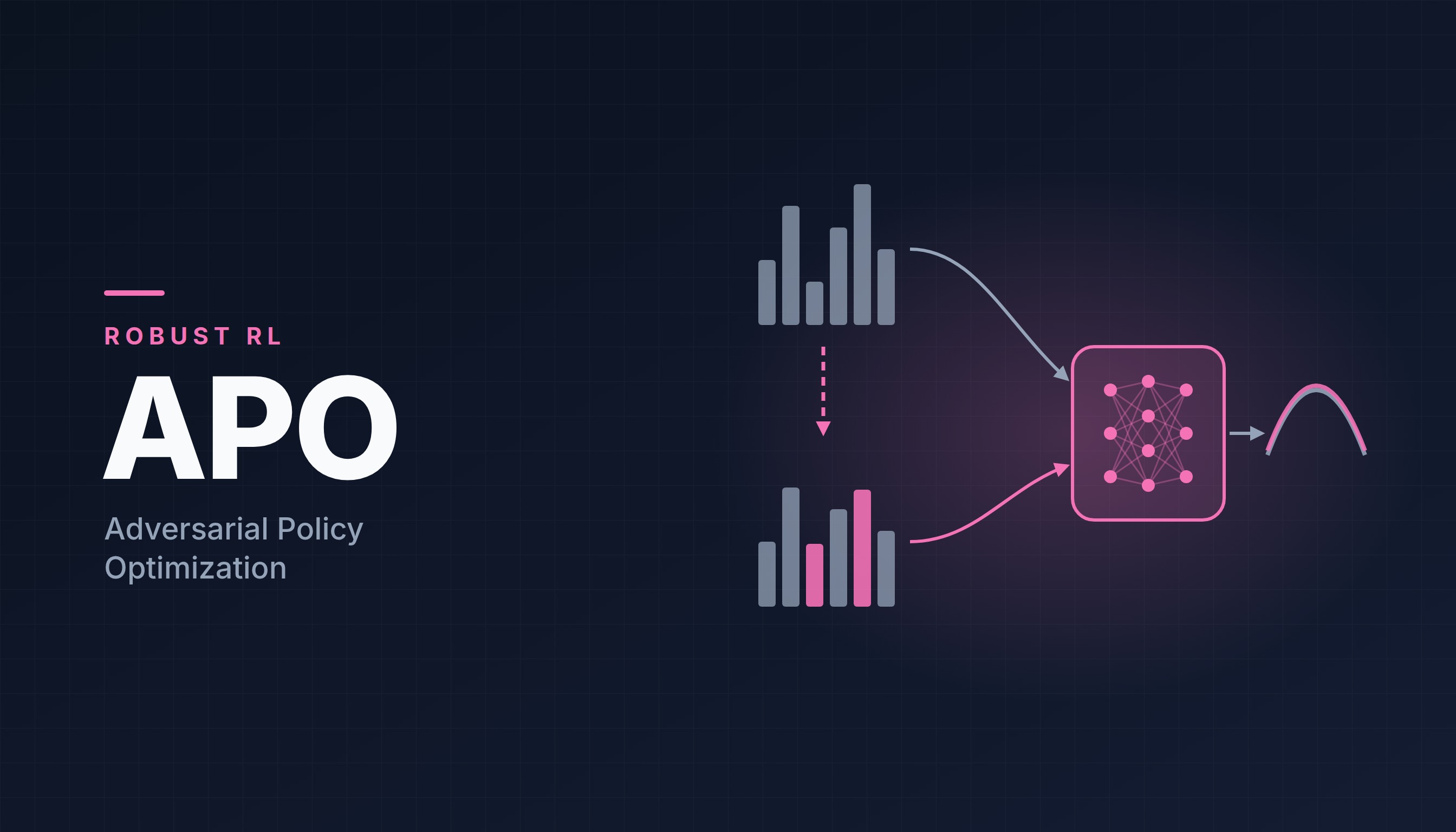
In 2023, Md Masudur Rahman and Yexiang Xue of Purdue University proposed APO (Adversarial Policy Optimization) [4], which learns the transformation instead of choosing it by hand. A second network, the perturber, learns to change the observation slightly in the way that changes the agent’s actions the most. The policy network, in turn, learns to keep its actions the same under those changes. The two networks play a max-min game, and the result is a policy that ignores the parts of the observation it should never have relied on. On the same Quadruped Run task, APO improved PPO by about $47%$ .

Unlike most posts here, APO is not about language models. It is a deep reinforcement learning method for continuous control, but it is built directly on PPO, and the adversarial idea is close to the one behind GAPO. In this post, we go through the PPO objective APO starts from, the perturber and the policy losses, and the training algorithm, and end with its limitations.

The Starting Point: PPO

At every timestep $t$ , the agent receives an observation $x_{t}$ , takes an action $a_{t}$ , and gets a reward $r_{t}$ . These play the roles of the state $s_{t}$ and the token $y_{t}$ in the PPO post. The paper uses the words state and observation for the same thing, since in its experiments the agent sees the full state vector. APO adds its adversarial terms on top of a base policy optimization method, and in the paper that method is PPO [5]. Written as a loss to minimize, the PPO objective is:

L_{π} = - E_{t} [\frac{π _{θ} ( a _{t} ∣ x _{t} )}{π _{θ_{old}} ( a _{t} ∣ x _{t} )} A_{t}] (1)

This is the probability-ratio surrogate from Eq. (10) of the PPO post, with a minus sign so that it can be minimized. The ratio compares the current policy $π_{θ}$ with the policy $π_{θ_{old}}$ that collected the data, and the advantage $A_{t}$ says how much better the action turned out than expected. As in Eq. (2) of the PPO post, it is the action value minus the state value:

A_{t} = Q (x_{t}, a_{t}) - V (x_{t})

Both are measured in terms of the return $G_{t}$ , the discounted sum of the rewards from step $t$ onward, as in Eq. (3) of the PPO post, with $γ = 0.99$ in the paper:

G_{t} = r_{t} + γ r_{t + 1} + γ^{2} r_{t + 2} + \dots = k = 0 \sum \infty γ^{k} r_{t + k}

The two halves are estimated exactly as in the PPO post. The return the agent actually collected after taking $a_{t}$ is one sample of $Q (x_{t}, a_{t})$ . $V (x_{t})$ comes from a value network, trained with the mean squared error of Eq. (4) of the PPO post to predict the average return, $V (x_{t}) = E [G_{t} ∣ x_{t}]$ , as in Eq. (5) of the PPO post.

There is one problem. PPO collects data in rollouts of a fixed length, $2048$ steps in the paper, and the episode usually has not ended when the rollout stops at step $T$ . The rewards up to $r_{T - 1}$ are known, but the rewards from step $T$ onward were never observed. So we split the return at step $T$ into the part we saw and the part we did not:

G_{t} = observed k = 0 \sum T - t - 1 γ^{k} r_{t + k} + not observed k = T - t \sum \infty γ^{k} r_{t + k}

In the second sum, every term carries at least $γ^{T - t}$ . Taking it out, and counting from step $T$ with $j = k - (T - t)$ , leaves exactly the return from step $T$ :

k = T - t \sum \infty γ^{k} r_{t + k} = γ^{T - t} j = 0 \sum \infty γ^{j} r_{T + j} = γ^{T - t} G_{T}

$G_{T}$ is unknown, but its expected value is exactly what the value network predicts, $V (x_{T}) = E [G_{T} ∣ x_{T}]$ . Replacing $G_{T}$ with $V (x_{T})$ , and writing out the observed sum, gives the estimate of the action value:

Q (x_{t}, a_{t}) \approx r_{t} + γ r_{t + 1} + \dots + γ^{T - t - 1} r_{T - 1} + γ^{T - t} V (x_{T})

If the episode did end before step $T$ , nothing comes after it, and $V (x_{T})$ is set to $0$ . This way of filling in the unseen future with a predicted value is called bootstrapping, as in the TD estimate of the PPO post.

Subtracting $V (x_{t})$ gives the advantage estimate used in the paper [4]:

A_{t} = - V (x_{t}) + r_{t} + γ r_{t + 1} + \dots + γ^{T - t - 1} r_{T - 1} + γ^{T - t} V (x_{T}) (2)

How far ahead the observed rewards reach decides what kind of estimate this is. If the rollout stops one step after $t$ , so that $T = t + 1$ , only one reward is observed, and Eq. (2) becomes:

A_{t} = r_{t} + γ V (x_{t + 1}) - V (x_{t})

which is the TD error from Eq. (7) of the PPO post. It relies mostly on the value network, so it has low variance but inherits the network’s errors. If instead the episode ends before $T$ , so that $V (x_{T}) = 0$ , every reward is observed, and it becomes the Monte Carlo estimate from Eq. (6) of the PPO post, which is unbiased but noisy. Eq. (2) lies between the two.

In the implementation, the ratio is clipped with $ϵ = 0.2$ , as in the clipped surrogate objective. And instead of a single estimate of Eq. (2), the advantage is computed with GAE, with $λ = 0.95$ , which averages such estimates over every lookahead [4]. Nothing in this part is new. APO’s contribution is what it adds to $L_{π}$ .

The Max-Min Game

APO trains two networks against each other. The perturber network, with parameters $ϕ$ , takes an observation $x$ and returns a perturbed observation $x^{'}$ . The policy network $π_{θ}$ is the agent itself. To measure how much the perturbation changes the agent’s behavior, APO compares the action distributions the policy gives for the two observations, $π_{θ} (\cdot ∣ x)$ and $π_{θ} (\cdot ∣ x^{'})$ , with the KL divergence.

The perturber wants this KL divergence to be large: it looks for a change to the observation that makes the agent act differently. The policy wants it to be small: it should act the same way whether or not the observation was perturbed. One side maximizes the same quantity that the other minimizes, which is what makes it a max-min game.

The Perturber Network

A perturber that is free to change anything would win easily. It could replace the observation with noise, and no policy could act the same on noise as on the real observation. So the perturber is also asked to keep its change small, measured by the squared $L_{2}$ distance between the two observations. Its loss is [4]:

L_{ϕ} = ∥ x_{t} - x_{t}^{'} ∥_{2}^{2} - KL (π_{θ} (\cdot ∣ x_{t}) ∥ π_{θ} (\cdot ∣ x_{t}^{'})) (3)

Minimizing the first term keeps the distortion small. Minimizing the second term, which has a minus sign, makes the KL divergence large. Together, the perturber is pushed toward the smallest change that moves the agent’s action the most. A small change that moves the action a lot is exactly a sign of overfitting. If a slight nudge to some features makes the agent behave very differently, the policy is relying heavily on those features.

The Policy Network

The policy network keeps learning from the reward with $L_{π}$ of Eq. (1), and adds the same KL divergence as a penalty [4]:

L_{θ} = L_{π} + KL (π_{θ} (\cdot ∣ x_{t}) ∥ π_{θ} (\cdot ∣ x_{t}^{'})) (4)

The KL term appears in Eq. (3) with a minus sign and in Eq. (4) with a plus sign. The perturber tries to make it larger, and the policy tries to make it smaller. For the policy, making it smaller means giving the same action distribution for $x$ and $x^{'}$ , which in turn means paying little attention to the features the perturber changed. Since the perturber always targets the features the policy is currently most sensitive to, the policy is steadily pushed away from relying on any small, easily changed part of the observation. The first term, meanwhile, keeps it learning the task.

This is how APO replaces a hand-chosen data augmentation. RAD decides in advance that, for example, scaling the observation should not change the action. APO lets the perturber find, at every step, the changes that the current policy is most vulnerable to. The two can also be combined: in the paper’s experiments, the observation is first scaled by a random factor between $0.6$ and $1.2$ , as in RAD, and then passed to the perturber and the policy [4].

The APO Algorithm

The two losses are minimized in turns. The agent first collects data with its current policy, then, for each collected observation, the perturber produces a perturbed observation, the policy is updated with Eq. (4), and the perturber is updated with Eq. (3) [4]:

Algorithm 1 Adversarial Policy Optimization

1 : 2 : 3 : 4 : 5 : 6 : 7 : 8 : 9 : 10 : 11 : initialize the policy parameters θ and the perturber parameters ϕ for each iteration do for each environment step do a_{t} \sim π_{θ} (a_{t} ∣ x_{t}) x_{t + 1} \sim P (x_{t + 1} ∣ x_{t}, a_{t}), r_{t} \sim R (x_{t}, a_{t}) D \leftarrow D \cup {(x_{t}, a_{t}, r_{t}, x_{t + 1})} for each observation x_{t} in D do x_{t}^{'} \leftarrow PerturberNetwork (x_{t}) compute L_{π} with PPO, Eq. (1) and Eq. (2) compute L_{θ} with Eq. (4) and update θ compute L_{ϕ} with Eq. (3) and update ϕ

Compared with PPO, the new parts are the perturber, in lines 1, 8, and 11, and the KL term inside line 10. The perturber is used during training only. At test time, the agent acts on the real observation, and the perturber is thrown away.

Limitations of APO

APO was tested only on vector observations, not on images, where data augmentation methods such as RAD are most often used, and only with PPO as the base algorithm. The APO agent in the experiments also used RAD’s random scaling, and the paper does not report APO without it, so how much of the gain comes from the adversarial game alone is not clear. The two terms of the perturber loss in Eq. (3), and the two terms of the policy loss in Eq. (4), are added with equal weight. The squared distance depends on the scale of the observation, so the balance between a small change and a large KL divergence may need tuning on other tasks. Finally, the gains vary a lot across random seeds, and on some tasks RAD or DRAC still did better.

APO showed that instead of guessing which changes to the observation should not matter, an agent can train against a network that searches for the changes it is most sensitive to, and learn to ignore them.

References

Song, X., Jiang, Y., Tu, S., Du, Y., & Neyshabur, B. (2020). Observational Overfitting in Reinforcement Learning. ICLR.
Laskin, M., Lee, K., Stooke, A., Pinto, L., Abbeel, P., & Srinivas, A. (2020). Reinforcement Learning with Augmented Data. NeurIPS.
Raileanu, R., Goldstein, M., Yarats, D., Kostrikov, I., & Fergus, R. (2020). Automatic Data Augmentation for Generalization in Deep Reinforcement Learning. arXiv:2006.12862.
Rahman, M. M., & Xue, Y. (2023). Adversarial Policy Optimization in Deep Reinforcement Learning. arXiv:2304.14533.
Schulman, J., Wolski, F., Dhariwal, P., Radford, A., & Klimov, O. (2017). Proximal Policy Optimization Algorithms. arXiv:1707.06347.

Navigation