Proximal Policy Optimization (PPO)

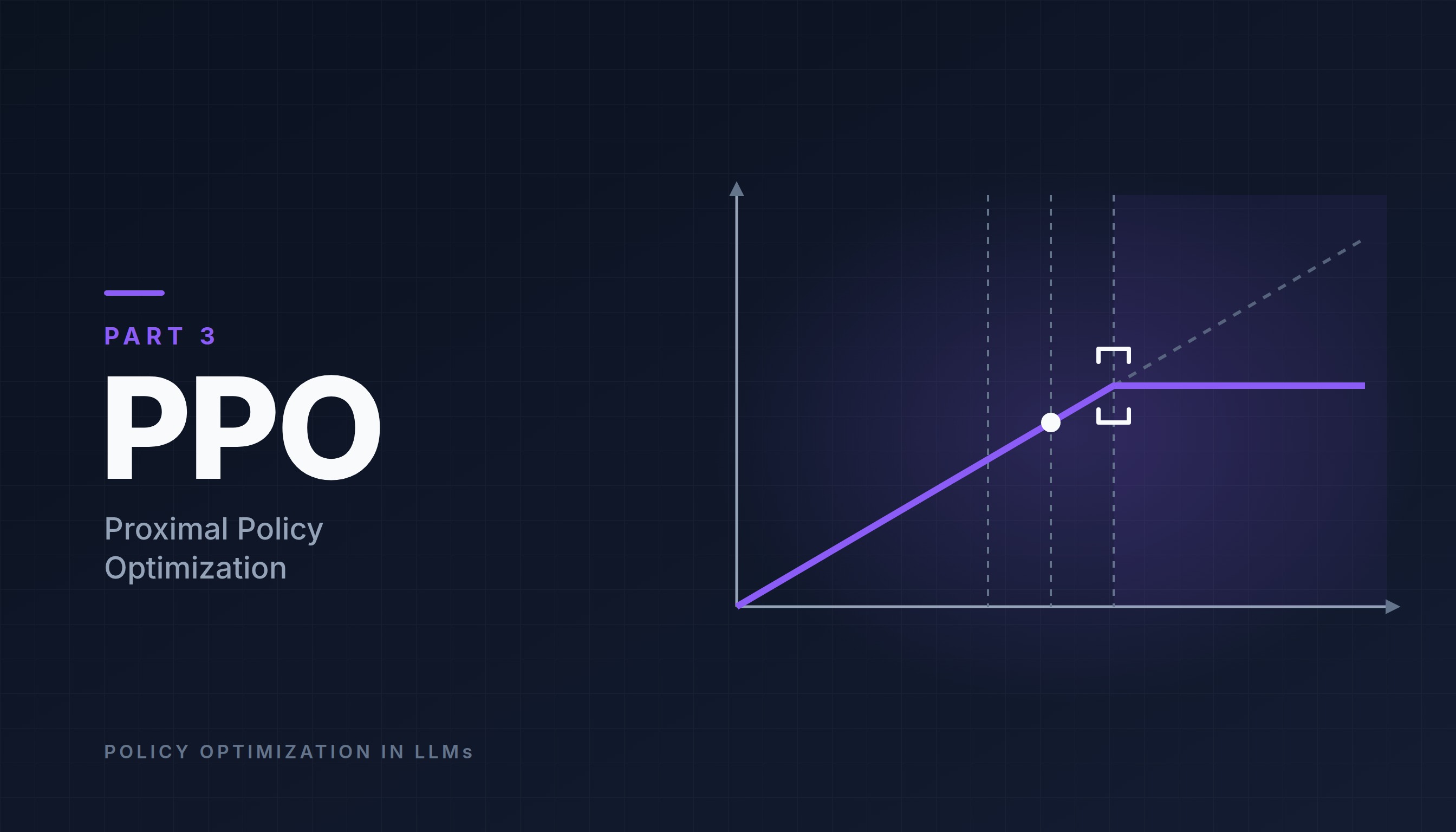
Introduction

Part 2 ended with an open question. TRPO made policy updates stable by keeping every step inside a trust region, but it achieved this stability with second-order optimization methods: the Fisher matrix, conjugate gradient, and a line search. All of this made each update expensive, hard to implement, and a poor fit for the way LLMs are usually trained. The question was whether we could get the same stability with ordinary first-order gradient descent.

In 2017, Proximal Policy Optimization (PPO) [1] answered yes. Instead of solving a constrained problem, PPO changes the objective itself so that the model gains nothing from moving too far. This idea is expressed in a single equation, the clipped surrogate objective, and it can be optimized with the same tools used to pre-train and fine-tune LLMs: mini-batches, a few epochs, and the Adam optimizer [2]. PPO matched or outperformed TRPO on standard benchmarks while being considerably simpler [1], and a few years later it became the algorithm behind the first instruction-following chat assistants [3].

To understand PPO properly, though, we first need to examine the quantity on which everything depends: the advantage $A_t$. In Part 1 we used a simple version of it, and in Part 2 we assumed it was given. This post therefore starts by examining where it comes from. We first see why reinforcement learning needs a scaling factor at all, and why that factor is the advantage. Computing the advantage then leads us, one problem at a time, to the value model, Monte Carlo returns, temporal difference (TD) bootstrapping, and finally Generalized Advantage Estimation (GAE). With the advantage in hand, we return to TRPO’s question: how to reuse the same samples for several updates with the probability ratio, and how PPO’s clipping keeps those updates safe. We end with the full PPO objective and algorithm, and how PPO is used to train language models.

From Supervised Learning to Scaled Updates

We start from what we already know. In supervised learning, every input comes with the correct answer. For an LLM, this is SFT: given a state $s_t$ (the prompt and the tokens so far), we know the correct next token $y_t^{\ast }$, and we make it more likely by maximizing its log-probability, as in Eq. (1) in Part 1:

$$\text{SFT:}\log {\pi }_{\theta }(y_t^{\ast }\mid s_t)$$

In reinforcement learning, there is no correct answer to copy. The model picks a token $y_t$ by itself, finishes its response, and only then receives a reward telling it how good the whole response was. It does not know whether a different token would have been better. All it knows is how things turned out.

The policy gradient handles this with a small change: keep the same log-probability, but multiply it by a number that says how good the outcome was. The simplest choice is the reward $R$ itself:

$$\text{Policy gradient:}\log {\pi }_{\theta }(y_t\mid s_t)\cdot R$$

When $R$ is positive, this behaves exactly like SFT: the sampled token becomes more likely. When $R$ is negative, it does the opposite and makes the token less likely. In other words, the reward acts as a scaling factor: it decides how strongly, and in which direction, the probability of the sampled token is pushed. The bigger the scaling factor, the bigger the push.

Using the raw reward as the scaling factor has a serious problem, though: it does not tell us whether the outcome was better than usual.

So instead of the raw reward, we scale by how much better or worse than expected the outcome was. That quantity is the advantage $A_t$, and it gives the policy gradient we already met in Eq. (2) in Part 1:

$$\text{Advantage policy gradient:}\log {\pi }_{\theta }(y_t\mid s_t)\cdot A_t\text{\hspace{1em}(1)}$$

Subtracting the expected outcome does not change the direction of learning on average, but it makes the scaling factor much less noisy, an idea known as using a baseline [4]. The next section answers one question: how do we actually compute $A_t$?

The Advantage Function

The advantage is the scaling factor that tells the model how strongly to push each token up or down, so everything PPO does depends on how well it is computed. In this section, we build it step by step. We first make “better than expected” precise, which shows that we need two quantities: what actually happened after a token, and what was expected to happen. We then see how each of them is measured, and how combining them gives three ways of estimating the advantage, each fixing a weakness of the previous one.

What “Better Than Expected” Means

To compute the advantage, we need to make “better than expected” precise. It compares two quantities, both measured as the total future reward from time step $t$ onward, called the return:

• $Q(s_t,y_t)$, the action value: the expected return if, in state $s_t$, we pick the specific token $y_t$ and then continue as usual. This is “how well things went with this token”, like your own exam score.
• $V(s_t)$, the state value: the expected return from state $s_t$ on average, over all the tokens the model might pick there. This is “how well things usually go from here”, like the class average.

The advantage is their difference:

$$A(s_t,y_t)=Q(s_t,y_t)-V(s_t)\text{\hspace{1em}(2)}$$

If picking $y_t$ leads to a better outcome than the average from $s_t$, the advantage is positive and the token is pushed up. If it leads to a worse outcome, the advantage is negative and the token is pushed down. If it is exactly average, the advantage is zero and nothing changes.

For example, in the state “What is 2 + 2? The answer is”, the average outcome is already good, because most tokens the model would pick here lead to a correct answer, so $V(s_t)$ is high. Picking the token “4” is even better than that average, so its advantage is positive. In a state like “What is 2 + 2? beep boop”, the response has already gone wrong, so $V(s_t)$ is low.

The problem is that we know neither $Q$ nor $V$. We have to estimate both, and the rest of this section follows that search step by step. We start with the more concrete half: what actually happened after the model picked $y_t$.

Measuring What Actually Happened: The Return

What happened after a token depends on the rewards the model received afterward. At each step $t$, the model receives an immediate reward $r_t$. PPO itself does not specify where these rewards come from; it only needs a number for each step. In the original PPO paper, the rewards came directly from the environment, such as the score in a game. For LLMs, they usually come from one of three sources:

• Sparse rewards from a checker. Every token gets $r_t=0$, except the last one, which gets the reward for the whole response, for example $+1$ if a math answer is correct and $0$ otherwise. This is the most common case.
• A reward model. When the goal is to follow human preferences and no automatic checker exists, a separate LLM trained on those preferences scores the finished response [3]. Its score is again given at the last token. This combination of PPO with a reward model is Reinforcement Learning from Human Feedback (RLHF), the topic of Part 4.
• A process reward model. For step-by-step reasoning, a model can score each intermediate step, giving rewards in the middle of the response as well [5].

In the most common cases, the reward only arrives at the very end. So to find out what a single token led to, we have to wait until the model finishes the full response, collect all the rewards, and add them up. This sum is the return, and each future reward is multiplied by a discount factor $\gamma$ (between $0$ and $1$) once for every step it lies in the future:

$$G_t=r_t+\gamma r_{t+1}+{\gamma }^2{r}_{t+2}+\cdots +{\gamma }^{T-t}{r}_T\text{\hspace{1em}(3)}$$

With $\gamma =0.9$, for example, the reward one step ahead counts $0.9$, two steps ahead $0.81$, three steps ahead $0.729$, and so on: the further away a reward is, the less it counts now. This is the decay. For LLM training, $\gamma$ is often set to $1$, so that the final reward counts fully for every token.

$G_t$ is the outcome that actually followed the token $y_t$, so it is a direct sample of $Q(s_t,y_t)$. That gives us the first half of the advantage. For the second half, $V(s_t)$, a single response is not enough: we need the average outcome from $s_t$.

Measuring What Was Expected: The Value Model

In principle, we could get $V(s_t)$ by stopping at state $s_t$, letting the model finish the response many times in different ways, and averaging the returns. But we would have to do this for every state of every response, which would multiply the cost of generation many times over. So instead of computing the average directly, we train a model to predict it. This model is the value model $V_{\varphi }$, also called the critic. The model that generates text, ${\pi }_{\theta }$, is then called the actor, and together they form an actor-critic setup [6].

For LLMs, the value model is itself an LLM. It reads the same text as the actor, but its last layer is different (Figure 1). The actor ends with a language-model head, which outputs a probability for every token in the vocabulary. The value model replaces it with a value head, a single linear layer that outputs one number: the estimate $V_{\varphi }(s_t)$.

The value model does not start from scratch. Its backbone is usually initialized from an existing model, such as the SFT model or the reward model (InstructGPT, for example, initialized it from the reward model [3]), so it already understands language. What it still has to learn is how much reward each state tends to lead to, and the returns we just computed are exactly what it needs. Every time the actor finishes a response, we know the real return $G_t$ for every step, and we train the value model to predict it with a mean squared error loss:

$$L^{\text{VF}}(\varphi )={\mathbb{E}}_t\left[\right(V_{\varphi }(s_t)-G_t{)}^2]\text{\hspace{1em}(4)}$$

Each individual $G_t$ is the outcome of one particular response, but over many responses, the prediction that minimizes this loss is the average return from each kind of state:

$$V(s_t)=\mathbb{E}[G_t\mid s_t]\text{\hspace{1em}(5)}$$

This also answers a natural question: how can the value model predict the future reward from a state like “The”, when it does not even know how many tokens are still to come? It does not need to. A strong chess player can look at a board and say “white wins this about 80% of the time” without knowing whether the game will last 10 or 50 more moves. They have seen many similar positions. In the same way, the value model has seen many responses that started like this one. And because it learns to predict $G_t$, which is already discounted, its estimates carry the same decay.

We now have both halves of Eq. (2): a sample of $Q$ from the return, and an estimate of $V$ from the value model. Putting them together gives our first estimate of the advantage.

First Estimate: Monte Carlo

The most direct estimate takes the definition of the advantage in Eq. (2) and replaces $Q(s_t,y_t)$ with the return $G_t$ that actually followed, from Eq. (3), and $V(s_t)$ with the value model’s estimate $V_{\varphi }(s_t)$. Since $G_t$ adds up the rewards of all the remaining tokens, it can only be computed after the model has generated every token of the response:

$${\hat{A}}_t^{\text{MC}}=G_t-V_{\varphi }(s_t)\text{\hspace{1em}(6)}$$

This is called the Monte Carlo estimate. The name comes from the Monte Carlo casino in Monaco. In the 1940s, mathematicians began solving hard problems by running many random trials and averaging the results instead of deriving an exact formula, and the method was named after the casino because it relies on chance, like games of chance [7]. Here, every finished response is one random trial.

Because $G_t$ uses only real rewards, this estimate has low bias: on average it is correct. But it has two problems. First, we still have to wait until the response is finished before we can compute anything. Second, and more importantly, it has high variance. $G_t$ depends on every random token sampled after step $t$, so a single unlucky choice later in the response changes it completely. If the model writes a perfectly good “The answer is” and then samples “5” instead of “4”, the return is $0$, and the good tokens at the start are blamed for a mistake they did not make. Over many responses this averages out, but each individual estimate is very noisy.

This raises a natural idea. We already have a model that predicts the future: the value model. Instead of waiting for the real future, which is noisy, why not ask the value model about it?

Second Estimate: TD Bootstrapping

Temporal difference (TD) bootstrapping does exactly that. To see how, write the Monte Carlo advantage with the return fully expanded:

$${\hat{A}}_t^{\text{MC}}=r_t+\underset{\text{replaced by }\gamma V_{\varphi }(s_{t+1})}{\underbrace{\gamma r_{t+1}+{\gamma }^2{r}_{t+2}+\cdots +{\gamma }^{T-t}{r}_T}}-V_{\varphi }(s_t)$$

Everything after the first reward is the return from the next step onward, multiplied by $\gamma$, that is, $\gamma G_{t+1}$. And the average of $G_{t+1}$ is exactly what the value model predicts for the next state, $V_{\varphi }(s_{t+1})$. So TD bootstrapping keeps only the immediate reward $r_t$, which is observed right away, and replaces the rest of the future with $\gamma V_{\varphi }(s_{t+1})$. This gives the TD estimate of the advantage. Because it is used so often, it has its own symbol, ${\delta }_t$, and its own name, the TD error:

$${\hat{A}}_t^{\text{TD}}={\delta }_t=r_t+\gamma V_{\varphi }(s_{t+1})-V_{\varphi }(s_t)\text{\hspace{1em}(7)}$$

Two names describe this idea. It is a temporal difference because it compares the value model’s estimates at two consecutive times, $t$ and $t+1$ [8]. And it is called bootstrapping, from the phrase “to pull yourself up by your own bootstraps”, because the value model uses one of its own estimates, $V_{\varphi }(s_{t+1})$, to improve another one, $V_{\varphi }(s_t)$, without waiting for the real outcome.

This fixes both problems of Monte Carlo. We no longer need to wait for the response to finish, and since only one random step is involved, the TD error has low variance: an unlucky token later in the response no longer affects the advantage of “The” directly. But it introduces a new problem. The TD estimate is only as good as the value model: if $V_{\varphi }(s_{t+1})$ is wrong, for example if it predicts $0.9$ when the true average is $0.6$, then ${\delta }_t$ is off by the same amount, and the advantage pushes the token in the wrong direction or by the wrong amount. A systematic error of this kind is called bias, so TD bootstrapping has high bias.

A daily-life comparison, adapted from Sutton and Barto [4], makes the trade-off concrete. Suppose you want to learn how long your commute home takes. With Monte Carlo, you only learn once you arrive: it took 45 minutes. One accident on the road makes that day’s number very different (high variance). With TD bootstrapping, you update along the way: you expected 30 minutes in total, and after 10 minutes you encounter heavy traffic and now expect 25 more. Your new estimate is $10+25=35$, five minutes more than before, and you can learn from that difference immediately. But if your “25 more minutes” guess is wrong, you learn the wrong thing (bias).

	Monte Carlo	TD bootstrapping
How much future is observed	The whole response	One step
How the rest is filled in	Nothing to fill in	With $V_{\varphi }(s_{t+1})$
Must wait for the response to finish	Yes	No
Bias	Low	High
Variance	High	Low

So each estimate fixes the other’s weakness, and neither is good enough on its own. But they are not the only two options. They are the two ends of a whole range of estimates. TD bootstrapping trusts the real reward for one step and the value model for everything after it. Monte Carlo trusts the real rewards for every step. In between, we can trust the real rewards for $n$ steps and the value model after that, which gives the n-step estimates of $Q$:

$$\begin{array}{rl}{\hat{Q}}^{(1)}(s_t,y_t)& =r_t+\gamma V_{\varphi }(s_{t+1})\text{(TD: low variance, high bias)}\\ {\hat{Q}}^{(2)}(s_t,y_t)& =r_t+\gamma r_{t+1}+{\gamma }^2{V}_{\varphi }(s_{t+2})\\ {\hat{Q}}^{(3)}(s_t,y_t)& =r_t+\gamma r_{t+1}+{\gamma }^2{r}_{t+2}+{\gamma }^3{V}_{\varphi }(s_{t+3})\\ & ⋮\\ {\hat{Q}}^{\text{MC}}(s_t,y_t)& =r_t+\gamma r_{t+1}+\cdots +{\gamma }^{T-t}{r}_T\text{(MC: high variance, low bias)}\end{array}$$

Moving down the list, each estimate uses one more real reward and relies one step less on the value model. That reduces the bias, but every extra real reward depends on one more randomly sampled token, which increases the variance. Subtracting $V_{\varphi }(s_t)$ from each of these gives the n-step advantages:

$$\begin{array}{rl}{\hat{A}}_t^{(1)}& =r_t+\gamma V_{\varphi }(s_{t+1})-V_{\varphi }(s_t)\\ {\hat{A}}_t^{(2)}& =r_t+\gamma r_{t+1}+{\gamma }^2{V}_{\varphi }(s_{t+2})-V_{\varphi }(s_t)\\ {\hat{A}}_t^{(3)}& =r_t+\gamma r_{t+1}+{\gamma }^2{r}_{t+2}+{\gamma }^3{V}_{\varphi }(s_{t+3})-V_{\varphi }(s_t)\\ & ⋮\\ {\hat{A}}_t^{\text{MC}}& =r_t+\gamma r_{t+1}+\cdots +{\gamma }^{T-t}{r}_T-V_{\varphi }(s_t)\end{array}$$

The first one is the TD error ${\delta }_t$ from Eq. (7), and the last one is the Monte Carlo advantage. The question is which $n$ to choose. A small $n$ is stable but trusts the value model too much; a large $n$ is accurate on average but noisy. The best choice depends on how good the value model is, and that changes during training. So instead of committing to a single $n$, what if we could use all of them at once, giving most weight to the stable short estimates while still letting the longer, more accurate ones contribute? This is exactly what Generalized Advantage Estimation (GAE) does.

Generalized Advantage Estimation

GAE [9] does not pick one $n$. Instead, it takes an exponential moving average (EMA) of all the n-step advantages. The 1-step advantage gets weight $1$, and each longer one gets $\lambda$ times the weight of the previous one, for a parameter $\lambda$ between $0$ and $1$. As in any weighted average, we multiply each estimate by its weight, add them up, and divide by the sum of the weights:

$${\hat{A}}_t^{\text{GAE}}=\frac{{\hat{A}}_t^{(1)}+\lambda {\hat{A}}_t^{(2)}+{\lambda }^2{\hat{A}}_t^{(3)}+\dots }{1+\lambda +{\lambda }^2+\dots }$$

The denominator is a geometric series, $1+\lambda +{\lambda }^2+\cdots =\frac{1}{1-\lambda }$, so dividing by it is the same as multiplying by $(1-\lambda )$:

$${\hat{A}}_t^{\text{GAE}}=(1-\lambda )({\hat{A}}_t^{(1)}+\lambda {\hat{A}}_t^{(2)}+{\lambda }^2{\hat{A}}_t^{(3)}+\dots )$$

Written this way, we would have to compute every n-step advantage separately. But each of them can be written using only TD errors. The 1-step advantage is the TD error itself, ${\hat{A}}_t^{(1)}={\delta }_t$. For the 2-step advantage, we add and subtract $\gamma V_{\varphi }(s_{t+1})$ and group the terms into two TD errors:

$$\begin{array}{rl}{\hat{A}}_t^{(2)}& =r_t+\gamma r_{t+1}+{\gamma }^2{V}_{\varphi }(s_{t+2})-V_{\varphi }(s_t)\\ & =(r_t+\gamma V_{\varphi }(s_{t+1})-V_{\varphi }(s_t))+\gamma (r_{t+1}+\gamma V_{\varphi }(s_{t+2})-V_{\varphi }(s_{t+1}))\\ & ={\delta }_t+\gamma {\delta }_{t+1}\end{array}$$

Doing the same for the longer estimates, each extra step adds one more TD error. So the list of n-step advantages becomes:

$$\begin{array}{rl}{\hat{A}}_t^{(1)}& ={\delta }_t\\ {\hat{A}}_t^{(2)}& ={\delta }_t+\gamma {\delta }_{t+1}\\ {\hat{A}}_t^{(3)}& ={\delta }_t+\gamma {\delta }_{t+1}+{\gamma }^2{\delta }_{t+2}\\ & ⋮\\ {\hat{A}}_t^{\text{MC}}& ={\delta }_t+\gamma {\delta }_{t+1}+\cdots +{\gamma }^{T-t}{\delta }_T\end{array}$$

Putting these into the EMA:

$$\begin{array}{rl}{\hat{A}}_t^{\text{GAE}}=(1-\lambda )(& {\delta }_t\\ +& \lambda ({\delta }_t+\gamma {\delta }_{t+1})\\ +& {\lambda }^2({\delta }_t+\gamma {\delta }_{t+1}+{\gamma }^2{\delta }_{t+2})+\dots )\end{array}$$

Now we collect the terms for each TD error. ${\delta }_t$ appears in every estimate, $\gamma {\delta }_{t+1}$ in every estimate from the second one on, and ${\gamma }^2{\delta }_{t+2}$ from the third one on. Each sum of weights is a geometric series like the one above:

$$\begin{array}{rl}{\hat{A}}_t^{\text{GAE}}& =(1-\lambda ){\delta }_t(1+\lambda +{\lambda }^2+\dots )\\ & +(1-\lambda )\gamma {\delta }_{t+1}(\lambda +{\lambda }^2+\dots )\\ & +(1-\lambda ){\gamma }^2{\delta }_{t+2}({\lambda }^2+\dots )+\dots \\ & =(1-\lambda ){\delta }_t\frac{1}{1-\lambda }\\ & +(1-\lambda )\gamma {\delta }_{t+1}\frac{\lambda }{1-\lambda }\\ & +(1-\lambda ){\gamma }^2{\delta }_{t+2}\frac{{\lambda }^2}{1-\lambda }+\dots \\ & ={\delta }_t+\gamma \lambda {\delta }_{t+1}+(\gamma \lambda {)}^2{\delta }_{t+2}+\dots \end{array}$$

The $(1-\lambda )$ cancels completely. After the last token there are no more TD errors, so the sum ends with ${\delta }_T$. This is the form of GAE used in practice: a sum of the TD errors of all future steps, where each one gets a weight that shrinks by a factor of $\gamma \lambda$ for every step it lies ahead:

$${\hat{A}}_t^{\text{GAE}}=\sum _{l=0}^{T-t}(\gamma \lambda {)}^l{\delta }_{t+l}\text{\hspace{1em}(8)}$$

The parameter $\lambda$ decides how far into the future we trust the real rewards, and its two extremes are exactly the two estimates we started with:

• With $\lambda =0$, only the first term remains: ${\hat{A}}_t={\delta }_t$, the pure TD bootstrapping estimate.
• With $\lambda =1$, every TD error until the end of the response is kept with weight ${\gamma }^l$. This is exactly ${\hat{A}}_t^{\text{MC}}$ from the list above, $G_t-V_{\varphi }(s_t)$, the pure Monte Carlo estimate.

Values in between trade a small increase in bias for a large reduction in variance. A common choice is $\lambda =0.95$. In practice, GAE is computed backward from the last token with a simple recursion, ${\hat{A}}_t={\delta }_t+\gamma \lambda {\hat{A}}_{t+1}$, starting from ${\hat{A}}_T={\delta }_T$.

Reusing Samples: The Probability Ratio

We now know how to compute the advantage for every token, so we can put the pieces together. Training the policy with the policy gradient from Eq. (1) and the value model with the loss from Eq. (4) looks like Algorithm 1:

Each pass through this loop is called an iteration. In every iteration, the batch ${\mathcal{D}}_n$ is used for a single update and then thrown away, because the policy gradient needs responses from the current model. This is wasteful, since generating responses token by token is the most expensive part of RL for LLMs.

Does this sound familiar? We faced the same problem in Part 2, and there we did not generate new samples after every update. We reused the old ones with importance sampling: each token is reweighted by the probability ratio between the model being trained and the old model that generated it, as in Eq. (5) in Part 2:

$${\rho }_t(\theta )=\frac{{\pi }_{\theta }(y_t\mid s_t)}{{\pi }_{{\theta }_{\text{old}}}(y_t\mid s_t)}\text{\hspace{1em}(9)}$$

This gave us the surrogate objective from Eq. (6) in Part 2:

$$L(\theta )={\mathbb{E}}_t[{\rho }_t(\theta ){\hat{A}}_t]\text{\hspace{1em}(10)}$$

(The PPO paper [1] calls this $L^{\text{CPI}}$ and writes the ratio as $r_t(\theta )$. We keep ${\rho }_t$ to avoid confusion with the reward $r_t$.)

We can do exactly the same here. The model that generated the batch, ${\pi }_{{\theta }_n}$, becomes ${\pi }_{{\theta }_{\text{old}}}$, and the ratio takes care of the fact that the model being trained is no longer the one that generated the batch. So we no longer have to throw the batch away after one update. We can train on it the way we train on any supervised dataset: go over it several times, where each pass is called an epoch, taking one gradient step per mini-batch, as in Algorithm 2:

With $4$ epochs of $8$ mini-batches, one batch now gives $32$ updates instead of $1$. At the first update, ${\pi }_{\theta }$ and ${\pi }_{{\theta }_{\text{old}}}$ are the same model, so every ratio is $1$. Over the epochs, the ratios drift away from $1$, and at the next iteration they return to $1$. But as we saw in Part 2, the surrogate is only trustworthy while the ratios stay close to $1$. Maximizing it freely would push the ratios of good tokens up without limit and break the policy. TRPO prevented this with a KL constraint and second-order optimization. PPO prevents it with a much simpler modification of the objective.

The Clipped Surrogate Objective

PPO keeps the surrogate objective, but removes the incentive to move the ratio far from $1$. It does this by clipping the ratio to the range $[1-ϵ,1+ϵ]$, where $ϵ$ is a small number, typically $0.2$:

$$L^{\text{CLIP}}(\theta )={\mathbb{E}}_t\left[\min \right({\rho }_t(\theta ){\hat{A}}_t,\text{clip}({\rho }_t(\theta ),1-ϵ,1+ϵ){\hat{A}}_t\left)\right]\text{\hspace{1em}(11)}$$

Here $\text{clip}(\rho ,1-ϵ,1+ϵ)$ means: if $\rho$ is below $1-ϵ$, use $1-ϵ$; if it is above $1+ϵ$, use $1+ϵ$; otherwise, use $\rho$ itself. With $ϵ=0.2$, the clipped ratio always stays between $0.8$ and $1.2$.

The objective takes the minimum of two terms: the normal surrogate ${\rho }_t{\hat{A}}_t$ and its clipped version. Taking the smaller of the two makes $L^{\text{CLIP}}$ a pessimistic estimate, a lower bound on the normal surrogate [1]. The model is never rewarded for pushing the ratio beyond the clipping range, but it is still penalized if a change makes things worse. Figure 2 shows what this looks like for a single token.

For each sign of the advantage, the figure has three regions, depending on which way the ratio has moved and how far:

	Harmful direction	Helpful direction, inside the range	Helpful direction, beyond the range
${\hat{A}}_t>0$ (good token)	${\rho }_t<1$: not clipped, gradient pushes ${\rho }_t$ back up	$1\le {\rho }_t\le 1+ϵ$: not clipped, gradient keeps pushing ${\rho }_t$ up	${\rho }_t>1+ϵ$: clipped, gradient is zero
${\hat{A}}_t<0$ (bad token)	${\rho }_t>1$: not clipped, gradient pushes ${\rho }_t$ back down	$1-ϵ\le {\rho }_t\le 1$: not clipped, gradient keeps pushing ${\rho }_t$ down	${\rho }_t<1-ϵ$: clipped, gradient is zero

Inside the range, the model learns exactly as with the normal surrogate, for good and bad tokens alike. Clipping only stops improvements that have already gone far enough, and it never stops the model from undoing a change that hurt. This is the sense in which PPO is “proximal”: the new model has no incentive to move more than about $ϵ$ away from the old one on any token.

The Full PPO Objective

The clipped objective improves the actor, but it relies on advantages that come from the critic. Since the actor changes after every batch, the returns it produces change too, so the critic must keep learning alongside it. PPO therefore trains the actor and the critic at the same time, and they can even share the same LLM backbone. TRPO could not handle this kind of parameter sharing, but PPO can, because everything is combined into a single loss minimized with gradient descent [1]. The full objective combines three terms:

$$L^{\text{CLIP+VF+S}}(\theta )={\mathbb{E}}_t[L_t^{\text{CLIP}}(\theta )-c_1{L}_t^{\text{VF}}(\theta )+c_{2}S[{\pi }_{\theta }](s_t)]\text{\hspace{1em}(12)}$$

• $L_t^{\text{CLIP}}$ is the clipped surrogate from Eq. (11), which improves the policy.
• $L_t^{\text{VF}}$ is the value loss from Eq. (4), which teaches the critic to predict returns. It is subtracted because the value error should be minimized while the rest is maximized.
• $S[{\pi }_{\theta }](s_t)$ is the entropy of the model’s next-token distribution, a measure of how spread out it is. Adding it as a bonus keeps the model from becoming too certain too early, which encourages exploration [6].

The coefficients $c_1$ and $c_2$ balance the three terms. The value loss is written with $\theta$ here because, when the actor and the critic share a backbone, the critic’s parameters are part of $\theta$. When they are separate LLMs, the value loss from Eq. (4) is minimized separately for $\varphi$.

The PPO Algorithm, Step by Step

Putting everything together, we can fill in the details of Algorithm 2. PPO alternates between collecting data and optimizing on it [1]:

1. Sample. Generate responses to a batch of prompts with the current model ${\pi }_{{\theta }_{\text{old}}}$, and store each token’s probability under that model.
2. Score. Compute the rewards $r_t$, for example with a checker or a reward model.
3. Estimate advantages. Run the value model on every state, compute the TD errors with Eq. (7), and the advantages with GAE, Eq. (8). Compute the returns $G_t$ as targets for the value model.
4. Optimize. For $K$ epochs, split the batch into mini-batches and take gradient steps on the full objective in Eq. (12), using the Adam optimizer.
5. Repeat. Set ${\theta }_{\text{old}}\leftarrow \theta$ and go back to step 1.

Step 4 is where PPO differs most from the vanilla policy gradient in Algorithm 1. The same batch is reused for several epochs, and clipping is what makes that safe. Typical settings are $ϵ=0.2$, $\gamma =0.99$ (or $1$ for LLMs), $\lambda =0.95$, and a few epochs per batch [1].

PPO was not designed for LLMs. Its original paper tested it on simulated robotic control and Atari games, where it performed better than other online policy gradient methods such as TRPO and A2C (a synchronous version of A3C [6]), while being much simpler to implement [1].

PPO for Language Models

Moving from games and robots to language models changes the scale of the problem. When PPO is used to fine-tune an LLM, as in InstructGPT [3], every model involved is itself a large language model. In the RLHF setup, where rewards come from a reward model, up to four of them are needed at the same time:

Model	Role	Trained during PPO?
Policy (actor) ${\pi }_{\theta }$	Generates responses	Yes
Value model (critic) $V_{\varphi }$	Estimates $V(s_t)$ for the advantage	Yes
Reward model	Scores finished responses	No
Reference model ${\pi }_{\text{ref}}$	Frozen SFT model, used to keep the policy from drifting too far	No

Only the first two belong to PPO itself. The reward model and the reference model are added by RLHF, and they are the subject of the next part. With a checker instead of a reward model, PPO needs only the policy, the value model, and optionally the reference model. For now, the important point is that the value model is a full-size LLM of its own. It roughly doubles the memory and compute needed for training, and it has to learn alongside the policy.

Limitations of PPO

PPO is considerably simpler than TRPO, but it still has important limitations:

• The value model is expensive. For LLMs, the critic is as large as the policy, and its estimates are only as good as its training. A poor value model gives noisy or biased advantages.
• Clipping is only an approximate trust region. It removes the incentive to move far on each token, but it does not strictly bound the KL divergence between the old and new models. In practice, the policy can still drift further than $ϵ$ suggests [10].
• Many details matter. Studies of PPO have found that its performance depends heavily on implementation choices, such as how advantages are normalized and how the value loss is handled, sometimes more than on the clipping itself [10], [11].

PPO showed that a simple clipped objective, optimized with ordinary gradient descent, is enough to keep policy updates stable. The question it left behind was where the reward comes from when we want a model to follow human preferences.

This is the question RLHF answers, and it is the topic of Part 4.

References

1. Schulman, J., Wolski, F., Dhariwal, P., Radford, A., & Klimov, O. (2017). Proximal Policy Optimization Algorithms. arXiv:1707.06347.
2. Kingma, D. P., & Ba, J. (2015). Adam: A Method for Stochastic Optimization. ICLR.
3. Ouyang, L., Wu, J., Jiang, X., et al. (2022). Training language models to follow instructions with human feedback. NeurIPS.
4. Sutton, R. S., & Barto, A. G. (2018). Reinforcement Learning: An Introduction (2nd ed.). MIT Press.
5. Lightman, H., Kosaraju, V., Burda, Y., et al. (2023). Let’s Verify Step by Step. arXiv:2305.20050.
6. Mnih, V., Badia, A. P., Mirza, M., et al. (2016). Asynchronous Methods for Deep Reinforcement Learning. ICML.
7. Metropolis, N., & Ulam, S. (1949). The Monte Carlo Method. Journal of the American Statistical Association, 44(247), 335–341.
8. Sutton, R. S. (1988). Learning to Predict by the Methods of Temporal Differences. Machine Learning, 3, 9–44.
9. Schulman, J., Moritz, P., Levine, S., Jordan, M. I., & Abbeel, P. (2016). High-Dimensional Continuous Control Using Generalized Advantage Estimation. ICLR.
10. Engstrom, L., Ilyas, A., Santurkar, S., et al. (2020). Implementation Matters in Deep Policy Gradients: A Case Study on PPO and TRPO. ICLR.
11. Huang, S., Noukhovitch, M., Hosseini, A., Rasul, K., Wang, W., & Tunstall, L. (2024). The N+ Implementation Details of RLHF with PPO: A Case Study on TL;DR Summarization. arXiv:2403.17031.